A Post by René Mõttus
Applying correlations that usefully describe trends in the population to individuals can often lead to incorrect conclusions. In individuals, high (as opposed to medium or low) values of one variable typically do not go with high values of another variable, even if these variables have a sizeable correlation at the population level. Even more unpredictably, medium values of one variable are almost equally likely to go with low, medium or high values of another variable.
In psychological research, typical research findings describe statistical trends in the population, hence pertaining to an abstract average person. Many of these trends represent relations between variables, and their strengths can be expressed using a correlation coefficient, which can range from 0 (no relation at all) to 1 (a perfectly predictable relation).
However, how much can we use the statistical trends found in the population to say something about individuals? In other words, to what extent is the abstract average person that emerges from our typical research findings prototypical of actual individuals like you and me?
For example, highly conscientious people have, on average, a high level of job performance. Say, this correlation approaches .30, representing a relatively strong population-level trend because most associations reported in psychological research are smaller.
So, when we hire a highly conscientious person, we are likely to get a highly productive employee, right? At least, we may expect this with a higher-than-chance probability, being correct over 50% of the time. Right? It depends on how we look at it.
Binomial Effect Size Display
To estimate how likely we are to be correct in applying a population-level correlation between two variables to individuals, we can use an intuitively appealing method called the Binomial Effect Size Display (BESD). It is based on categorising people into binary groups in both variables and cross-tabulating the expected proportions of the four groups that emerge.
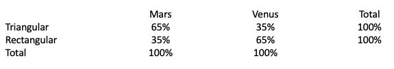
BESD works best for naturally binary variables, say living on Mars versus Venus or wearing triangular versus rectangular hats. In such cases, the proportions can be calculated by spreading the correlation coefficient equally around the random-guess value of .50, or 50% in the percentage scale.
If so, a hypothetical correlation of .30 between living on Mars and wearing a triangular hat will result in the proportion of .50 + (.30 / 2) = .65, or 65%, for the correlation-obeying individuals who either live on Mars and wear a triangular hat or live on Venus and wear a rectangular hat. In contrast, the proportion of the correlation-defying individuals who either live on Mars but wear a rectangular hat or live on Venus but wear a triangular hat would be .50 - (.30 / 2) = .35, or 35%.
To make BESD work for the continuously distributed variables typically used in personality research, such as conscientiousness and job performance, they must be collapsed into binary groups first. This can be done by splitting their distributions at their medians, forming “high” and “low” groups for both variables.
But this will typically reduce their correlation by over a third. As a result, the correlation .30 sinks to just below .20, and the proportion of correlation-obeying individuals is about 59.7%. This means that about 40.3% of individuals defy the population-level trend.

Figure 1. BESD for a correlation of .30 between two continuously distributed variables. The proportions should add up to 100% in both rows and columns (bar rounding error). If there was no correlation at all, all proportions would be 50%.
So, the answer to the question above would be yes: employing a person with an above-median conscientiousness score, we are likely to get an employee with above-median productiveness, about three times out of five.
Put differently, if we were to conclude that a person with below-median conscientiousness is unlikely to be performing that well at their job, we would be wrong two times out of five.
Limitations of using BESD
However, applying the BESD to correlations between continuously distributed variables has some limitations, in my view.
Even heuristically, people do not fall into just high and low groups for most variables that interest personality researchers. At the very least, many people score moderately in them because they aren’t consistently one way or another. For example, I am neither an extrovert nor introvert, but sometimes one, sometimes the other – call me an ambivert, if you will. Hence, I would score moderately in extraversion.
In fact, many variables used in personality research have bell-shaped distributions and therefore most people fall into a fairly limited range of values in the middles of these distributions, hovering just around the border between what would appear high and low values in BESD. So, many “highs” and “lows” are actually very similar to each other, perhaps indistinguishable to the naked eye and certainly more similar than each of them is too many of their fellow “highs” or “lows”.
Also, using BESD for such variables does not address a pervasive statistical phenomenon called regression to the mean: high (or low) values in one measurement are statistically expected to match relatively lower (or higher) values in another measurement, even when the variables are correlated. Even within high or low groups, people at the more extreme end in one variable are more likely to be closer to the middle in the other variable. And the more extreme one value is, the bigger the leap is towards the average that the other value is expected to take.
For example, a highly conscientious person is likely to regress towards the average on any other measure, even if they remain above the average – maybe just by a whisker. Because the high and low groups are so broad when using BESD for continuously distributed variables, this trend is masked.
Trinomial Effect Size Display
We may try extending the BESD to TESD, or the Trinomial Effect Size Display, and explore how this allows connecting population-level correlations with individuals. In short, this means putting people in three instead of two bins in each variable.
Of course, allocating people into three groups in otherwise continuously distributed variables is just as arbitrary as putting them into two bins, but it does allow for a bit more granularity – and some extra insights, as we will see. Besides, while dichotomising variables typically reduces correlations between them by over a third, collapsing them into three bins reduces their correlations only by about a fifth (because less information is filtered out from the variables).
For the easiest possible solution, we can set the three groups for each variable – low, medium and high – equal in size. Assuming bell-shaped distributions for the variables, the low and high groups comprise larger proportions of the variables’ ranges than the medium groups: this is because most people are in the middles of the distributions, whereas more extreme values are ever less common. The medium groups thus represent those hovering around the low-high borders in the BESD – many of whom are classified as different, but are actually very similar in the variables in question.[1]
To understand how TESD works, I simulated many pairs of such variables, only varying the correlations between them, collapsed each variable into three equally sized groups and cross-tabulated the proportions of observations for each of the nine possible combinations: low-low, low-medium, …, medium-high, high-high.
The R code for the simulations is here.[2]
Correlation .30
Let’s start with the correlation of .30, such as the one above, between conscientiousness and job performance. Such correlations are on the rarer side in psychology, representing “a large effect that is potentially powerful in both the short and the long-run” according to Funder and Ozer’s thoughtful effect size framework.
And yet, applying this correlation to individuals and expecting a high (or low) value to match another high (or low) value, we will be incorrect more often than not.
For example, someone with a high (or low) conscientiousness has about a 45.7% probability of having a high (or low) level of job performance and hence a 54.3% probability of having either regressed to the medium group or even slumped to the low-performance group.
[1] The TEDS will not behave very differently if we assume uniform distributions for the variables, in which case each group covers a similar range on each variable. If anything, the accuracy in applying correlations to individuals would be somewhat smaller than I show in my simulations based on normal distributions.
[2] In these examples, I assumed no measurement error, systematic or random. Adjusting for measurement error could make correlations larger, whereas error at the level of individual measurements would complicate applying correlations to individuals even more.
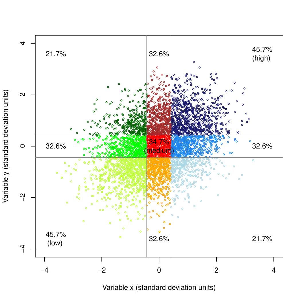
Figure 2. TESD for a correlation of .30 between two continuously distributed variables. The proportions should add up to 100% in both rows and columns (bar rounding error). If there was no correlation, all proportions would be 33.3%.
It will take a correlation of .40 for the probability that high (or low) values align to reach at least 50% – that is, for our expectation of matching high or low values to be correct at least at a random guess level. Such correlations, however, are rare in psychology: even some quite obvious ones, such as the correlation between low agreeableness and aggressive behaviour, do not reach that high.
For even higher and rarer correlations of .50 and .60, “highs” match “highs” and “lows” match “lows” 54.8% and 59.9% of the time, respectively. For example, if individuals’ standings in a trait correlate at .60 over several years, about three out of five of those scoring in the top third in the first occasion will stay there for the second testing as well, whereas about 40% are expected to become medium-scores or even score in the lowest third at the second testing.
More typical correlations
Coming back to more mundane numbers, one of the most typical effect sizes in psychology is a correlation around .20, such as the one between income and happiness.
Here, someone with a high (or low) score on one variable has about a 41.5% probability of also having a high (or low) score on another variable. So, expecting someone with a high income also to have a high happiness level, we will be wrong just under three times out of five.

Figure 3. TESD for a correlation of .20 between two continuously distributed variables. The proportions should add up to approximately 100% in both rows and columns (bar rounding error). If there was no correlation, all proportions would be 33.3%. If there was no correlation, all proportions would be 33.3%.
Next up, a correlation of .10 is on the smaller side but still common and “potentially … ultimately consequential”, according to Funder and Ozer. A suitable example of such a correlation is the widely publicised one between the growth mindset and academic performance.
According to TESD, a person with a high value on growth mindset has about 37.4% probability to also rank high in academic performance, hence having a 62.6% probability of having either regressed to the medium or even sunk to the low academic performance group.
In other words, applying the population-level correlation to individuals and expecting someone ranking high (or low) in growth mindset also to have high (or low) academic performance, we will be wrong over three times out of five.
This surely is not a conclusion worth making.
Some implications
Extending BESD to three levels instead of just low versus high – and calling it TESD, accordingly – has implications that may seem counter-intuitive at first. Even for relatively strong correlations according to reasonable standards in the field, a person with a high or low level in one variable is more likely to have a different level in another variable.
So, if we expect a person who has ranked high in a conscientiousness measure to also perform highly at the workplace (a known strong correlation), we will likely be disappointed.
There is, of course, a different way to look at this. When we don’t know anything about a person, there is a 33.3% probability of being correct when we put them in the top third of job performance. But knowing that the person scores in the top third in conscientiousness nudges this probability up to 41.5%. In other words, the probability of us being wrong to expect a person to have high job performance decreases from two thirds (a random guess) to under three out of five (knowing about their high conscientiousness). Of course, we would still be more often wrong than right.
Alternatively, we could take out those having a medium value on either variable and say with some conviction that a person with high conscientiousness is relatively unlikely to be among the bottom third in job performance. Here, we would be correct with about 67.8% probability (45.7 / (45.7 + 21.7)), hence beating the 50% guessing rate. That is, we would be correct over two times out of three -- and misclassify “only” a bit less than every third individual. But this can give us a distorted picture as we need to completely ignore over half the people because they have at least one medium value. Ignoring most individuals may work for candidate screening but not so much for interpreting research findings when we cannot chuck out data to make our findings look more impressive.
As a side note, interpreting correlations through TESD a positive upshot: someone very low in a desirable characteristic is likely to fare better in other desirable characteristics even when these characteristics are highly correlated in the population. For example, a low-conscientiousness person is likely to be more productive than you might think from the respective population-level trend and that kid with a very poor growth mindset is statistically unlikely to have low academic performance, all else equal.
Saying something about the folks in the middle
Unlike the BESD, the TESD allows us to see how well we can apply population-level correlations to say something about those with moderate levels in the variables. In short, we cannot say anything about them at all, really.
Even for sizeable correlations such as .30, people with medium levels in one variable are almost equally likely to be anywhere in the other variable’s distribution. That is, their probability of falling into the medium group in the other variable is about the same as the probability that they fall into either the high or low groups – the difference is only about two percentage points.
Why? Because observations regress towards the mean, moving from one measurement to another.
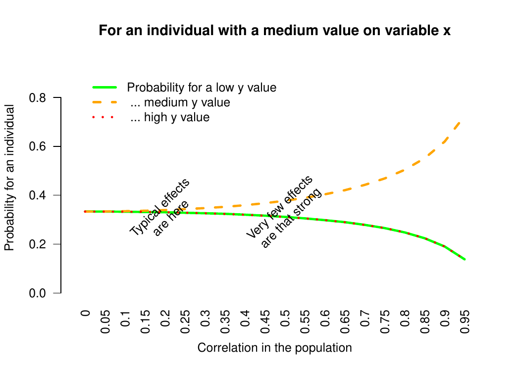
Figure 4. Probabilities that someone with a medium value in variable x also has a medium (as opposed to high or low) value in variable y, as a function of the correlation between x and y.
Calculate the TESD for your correlation
Because for typical correlations (up to .30) the medium levels in one variable are almost as likely to correspond to any levels in the other variable, you can calculate the approximate probability that a high (or low) value in one variable matches a high (or low) value in the other variable in a manner not very dissimilar to BESD.
First, multiply your correlation by .80 to account for the effect of putting people into three bins. Second, spread the correlation equally around the random-guess value of one third (1/3) to get the probabilities for matching (high-high, low-low) and mismatching (high-low, low-high) observations.
For a correlation of .30, it will be approximately 1/3 + (.30 * .80 / 2) = .453, or 45.3%, and 1/3 - (.30 * .80 / 2) = .213, or 21.3%.
But these are only approximations and work somewhat less well as correlations rise over .30. For example, for a correlation of .50, the approximation will underestimate “high-highs” by about 1.5%.
You can get more precise values for all correlations from here.
Or you may adapt the R code to calculate the TESD for any correlation.
Conclusion
Correlations are very useful for showing trends at the population level and allowing us to describe a hypothetical average person for our intellectual pleasure. Where necessary conditions are met, they may also allow for cost-effective population-level interventions. Yet, using them to draw categorical conclusions about particular individuals can be very, very tricky. More often than not, these conclusions can be misleading or even wrong. I hope that TESD helped to show you why.
We should therefore avoid generalising correlations beyond their purview – the hypothetical average person – to actual individuals. This hypothetical average person is just not prototypical enough of actual individuals. I am sure this has been said already a million times, but it cannot hurt to be reminded once again.
* I am grateful to Wendy Johnson, Lisanne de Moor and Yavor Dragostinov for their helpful comments.